Conditional formatting
In the ribbon start we find the menu for conditional formatting. Conditional formatting highlights cells depending on their content or a formula.
Excel already offers many common rules for highlighting cells. For our example the check for equal values is useful.
-
A dialog appears in which, starting from the selected cell, we first select the cell that is to be checked for the same values. Here this is cell D3, which contains the untranslated Magento constant in the Text column. IMPORTANT: Make sure that the reference is not set to absolute (cells preceded by $ signs). After that we still choose the type of highlighting: the default light red fill 2 format does the trick.
-
To apply this conditional formatting to all cells in the column, we switch back to the conditional formatting menu and open the "Manage rules" item.
-
In the column "is applied to" we now only enter the area to which the rule is to be applied. The easiest way to do this is to click in the first cell under the column header Translated and then press the down arrow while holding down the Shift and Control keys (Ctrl+Shift+Down Arrow). Excel will then automatically highlight to the bottom of the table.
-
With "OK" we close the dialog and can now view the result. All texts whose contents have not yet been changed are now highlighted in red. As soon as you translate the text, Excel automatically removes the highlighting.
Besides different colors, Excel also supports symbol sets and shapes. This looks even more concise and allows more variations.
- Start -> Conditional formatting -> Symbol sets
For certain shapes and symbols, the formulas for the conditions must be stored:
- Start -> Conditional formatting -> Manage rules -> Double click on the symbol set
Also cobby uses symbol sets of conditional formatting to show at a glance if the loaded data is still up-to-date. In this case means:
-
green = the data in Excel matches the data in Magento
-
yellow = the own changes have not been transferred to Magento yet
-
red = the data you see is out of date because either another user or Magento has changed it
This allows you to quickly see in real time whether you are editing outdated or current data. This makes it possible for several users to work in parallel.
To get the current status of all product data from Magento again, simply click on "Load products" under the "cobby" ribbon.
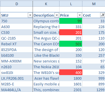
Often, with large amounts of data, we have the problem of quickly getting a correct feeling for a value. This is for example the case with the Ratio of purchase to sales price. To quickly create a visual aid here, conditional formatting is the first choice as in the following example:
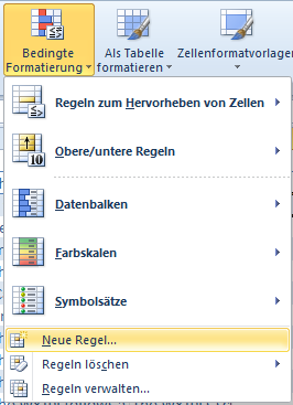
- It would be convenient if the price column is displayed in red when the margin is below 20%, for example, or in green when it exceeds 60%. To achieve this, we switch to the price column. Then we click on "Conditional formatting" -> "New rule" in the ribbon.
-
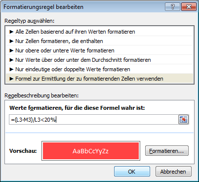
In the dialog we select Use formula to determine the cell to be formatted as the rule type. The formula we build must always return a result that is TRUE or FALSE.
-
In our example, we first determine the margin. In theory, the formula looks like this: (sales price-purchase price)/sales price. Transferred to our fields this means ( (L3-M3)/L3 ). Now, to get only one result of the type TRUE or FALSE, we use the operator
>and put the 60% into the formula: ( (L3-M3)/L3 > 60% ).
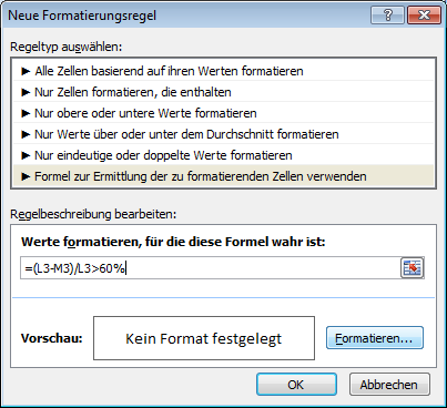
Please note: When the cells are selected with the mouse, the absolute formatting ($ - character) must be removed to be able to transfer the formula to other cells later. Then select a suitable formatting via the Format ... button (here a green background).
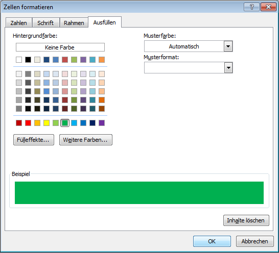
- To also highlight the margins that are too small, we go through the described steps again. For the formula, however, we now use the operator
<and insert 20% into the formula ( (L3-M3)/L3 < 20% ). As formatting we choose a red background with white font.
- In the last step, we still apply the formatting to the whole column and see at a glance which products have above or below average margins.
