How to use the VLOOKUP function to assign data
We have already learned how Excel and formulas can make our lives easier with Magento. Today we would like to introduce another important formula in Excel that every cobby user should know: the VLOOKUP. Before we start with our concrete example, we will briefly explain how VLOOKUP works.
It is described to do the following: "Searches the first column of a matrix and traverses the row to the right to return the value of a cell". The function comes with these parameters: =VLOOKUP( search_criterion ; matrix ; column_index ; range_reference )
The matrix in this case is the range from B3 to D7. Excel now always searches the 1st column of this matrix for the search criterion, i.e. the value we want to compare. It does this until the value is found or the end of the matrix is reached. If it finds a match for the search criterion (here: for the value 4), the VLOOKUP returns the value from the column index (here: 3).
Example: Assign prices
Step 1: Open supplier list
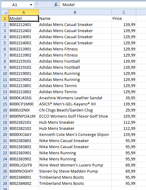
It often happens that we receive updates from suppliers in the area of item data, e.g. new prices. As long as our suppliers keep an indicator in their Excel list that we can compare with our products, the prices can be automatically assigned in Magento with cobby. To do this, we first open the supplier list.

Step 2: Sort from A to Z
It is important for the VLOOKUP that the matrix must be sorted by the first column. So, if not already done: We select the first row of the matrix and call the function "Sort from A to Z" in the ribbon Data.

Step 3: Load products
Afterwards we load the product data from Magento via "Load products".

Step 4: Enter VLOOKUP formula
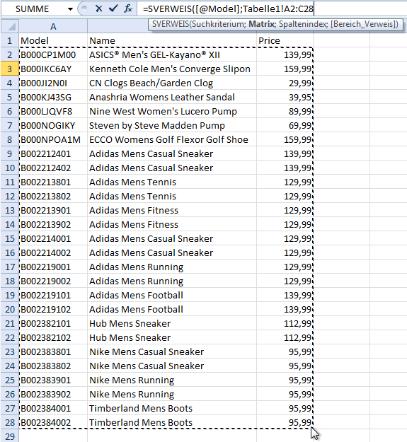
Now we switch to the cell into which we want to transfer a value from the manufacturer list. In our example, this is Price (remember: set the cell format to Standard so that the formula is calculated). Using the formula bar, we then enter the formula for the VLOOKUP. The search criterion that matches in the manufacturer list and in Magento is Model in our example (often the EAN).

Step 5: Mark the range for search
The matrix to be searched is located at the very end of the spreadsheets. There we now mark with the mouse the area that is to be searched.

Step 6: Enter parameter (value, exact match)
Now we determine which value is returned. Here it is the price in column 3 of the matrix, i.e. 3. As last parameter the VLOOKUP needs the indication whether an exact match must be found. Here, the option FALSE is nearly always entered. With closed parenthesis ) we confirm the formula.

Step 7: Set reference to matrix to absolute ($)
Before we can apply the formula to all other cells of this column, we have to set the reference to the matrix absolute. We do this by entering a dollar sign ($) in front of each cell.
