How to Use Conditional Formatting
Learn how to visually highlight cells based on their content or formulas using Excel's conditional formatting.
When to Use This
Use conditional formatting to:
- Highlight products that need attention
- Visualize profit margins
- Identify untranslated content
- Show stock levels at a glance
- Track data quality issues
Understanding Conditional Formatting
Conditional formatting changes cell appearance (color, icons, etc.) based on rules you define. It updates automatically as data changes.
Example 1: Highlight Untranslated Text
This example shows how to highlight cells that haven't been translated yet.
Step 1: Select the Cell
Click the first cell in your "Translated" column.
Step 2: Apply Conditional Formatting
- Go to Home ribbon
- Click Conditional Formatting
- Choose Highlight Cells Rules > Equal To
Step 3: Configure the Rule
In the dialog:
- Reference the untranslated text cell (e.g., D3)
- Important: Remove $ signs (absolute references) so the rule applies correctly to all cells
- Choose formatting (e.g., light red fill)
- Click OK
Step 4: Apply to All Cells
- Go to Conditional Formatting > Manage Rules
- In "Applies to", select the entire column range
- Click in the field and press Ctrl+Shift+Down Arrow to auto-select to the bottom
- Click OK
Now all untranslated cells are highlighted in red. When you translate the text, the highlighting automatically disappears.
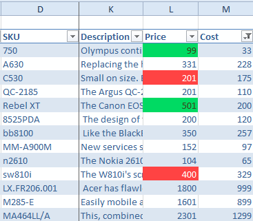
Example 2: Visualize Profit Margins
This example shows how to color-code products based on their profit margins.
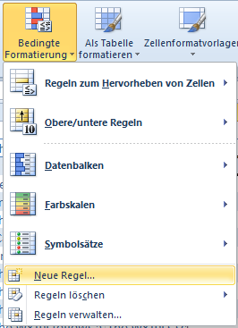
Step 1: Open Conditional Formatting Dialog
- Select the price column
- Go to Home > Conditional Formatting > New Rule
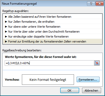
Step 2: Choose Formula Rule
Select Use formula to determine the cell to be formatted.
The formula must return TRUE or FALSE.
Step 3: Create High Margin Formula
For margins above 60% (green):
=(L3-M3)/L3 > 60%
What this does:
- (L3-M3) = Sales price minus purchase price
- Divided by L3 (sales price) = margin percentage
-
60% = returns TRUE if margin exceeds 60%
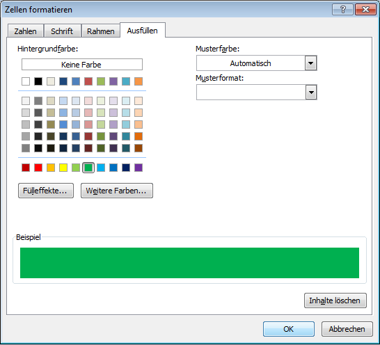
Step 4: Set Formatting
- Click Format...
- Choose green background
- Click OK
Important: Remove $ signs from cell references (L3, not $L$3) so the formula adjusts for each row.
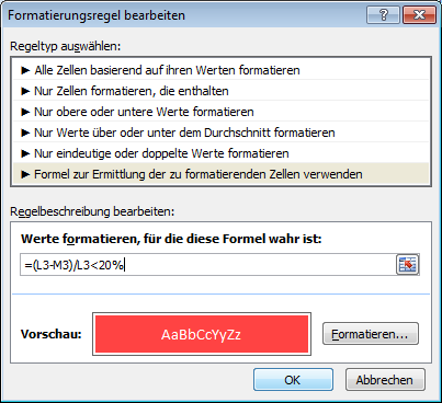
Step 5: Create Low Margin Formula
Repeat for margins below 20% (red):
=(L3-M3)/L3 < 20%
Choose red background with white font.
Step 6: Apply to All Rows
Copy the formatting down the entire column. Now you can see at a glance which products have good or poor margins.
Common Conditional Formatting Rules
Stock Levels
=[@Stock] < 10
Highlights products with low stock (red).
=[@Stock] > 100
Highlights well-stocked products (green).
Price Ranges
=[@Price] > 100
Highlights expensive products.
Empty Cells
=[@[Meta Description]] = ""
Highlights missing meta descriptions.
Duplicates
Use built-in rule:
- Conditional Formatting > Highlight Cells Rules > Duplicate Values
Date-Based
=[@[Special Price To Date]] < TODAY()
Highlights expired special prices.
Using Icon Sets
Icon sets display symbols instead of colors.
Step 1: Select Column
Select the column you want to format.
Step 2: Choose Icon Set
- Go to Home > Conditional Formatting > Icon Sets
- Choose a set (traffic lights, arrows, shapes, etc.)
Step 3: Configure Thresholds
- Go to Manage Rules
- Double-click the icon set rule
- Set formulas or values for each icon
- Click OK
cobby's Built-In Conditional Formatting
cobby uses conditional formatting to show data status:
- Green: Data matches Magento (up to date)
- Yellow: You have unsaved changes
- Red: Data is outdated (changed in Magento or by another user)
This helps you see at a glance when to reload or save products.
To refresh data, click Load products in the cobby ribbon.
Tips
- Remove $ signs: For formulas that apply to all rows, don't use absolute references
- Test first: Apply to one cell and verify it works
- Layer rules: Multiple rules can apply to the same cell (order matters)
- Clear formatting: Conditional Formatting > Clear Rules if you need to start over
- Copy formatting: Format Painter copies conditional formatting to other cells
Advanced: Symbol Sets with Formulas
For custom symbol conditions:
Step 1: Apply Symbol Set
- Select column
- Conditional Formatting > Icon Sets > Choose set
Step 2: Edit Rules
- Conditional Formatting > Manage Rules
- Double-click the symbol set
- Set conditions with formulas or percentages
- Click OK
Troubleshooting
Formatting not applying?
- Check that your formula returns TRUE/FALSE
- Test the formula in a cell:
=YOUR_FORMULAshould show TRUE or FALSE - Verify cell references are correct (relative vs absolute)
Wrong cells highlighted?
- Remove $ signs from formulas if rule should apply to all rows
- Check the "Applies to" range in Manage Rules
Formatting conflicts?
- Multiple rules may be competing
- Check rule order in Manage Rules (top rules take precedence)
- Use "Stop If True" to prevent lower rules from applying
Performance issues?
- Too many conditional formatting rules slow Excel
- Simplify rules or reduce the range they apply to
- Consider removing unused rules
Best Practices
Keep It Simple
- Use clear, obvious colors
- Don't over-format (too many colors confuse)
- Focus on actionable insights
Use Consistent Colors
- Red: Problems, errors, low values
- Yellow: Warnings, pending items
- Green: Good, complete, high values
Document Your Rules
Add a legend explaining what colors mean, especially if sharing files.